Voracious sort

Disclaimer: This article is part of a serie of articles about the Rust Voracious Radix Sort Crate. This article is about the Voracious sort inside the Voracious Radix Sort Crate, not the crate itself.

• What is radixsort ?
• Voracious sort
• Diverting LSD sort
• Rollercoaster sort: The best of the two worlds
• Peeka sort: Multithreaded radix sort – TBA –

For one of my previous work I needed a very fast sort in Rust, because the R&D was done in Rust. I looked for an already existing crate and I found nothing very interesting. The Rust standard library already provides the unstable_sort() which is the fastest sort available in Rust. Under the hood, the unstable_sort() is an implementation of the Pattern Defeating Quicksort invented and implemented by Orson Peters in C++ and implemented by Stjepan Glavina in Rust. It can be considered as the state of the art of the quicksort family. But I wanted something faster.

I searched on the Internet and I found the Ska sort on Malte Skarupke blog. I decided to implement it in Rust. Since it was my first time implementing a radix sort, I had to understand it first. Actually the Ska sort is an improvement of the American flag sort, which is an in place unstable non comparative sort.

« In place » means that the sort does not need extra memory: the space complexity is O(1). « Unstable » means that the sort can reorder a previous ordering. « Non comparative » means that the sort does not use a comparative function. For more explanation see here.

First, we have to understand how the American flag sort works to understand what is the improvement in the Ska sort and then to understand how Voracious sort is an improvement of the Ska sort.

Prerequisite

My previous article on radix sort: what is radixsort ?.

Level.

If you read my previous article on the radix sort, you should understand what is the radix. Most of the time, the best radix is 8. It is the best trade-off between the number of passes and the required memory.

If you divide a 32 bits number into chunks of 8 bits, you will end up with 4 levels. By my own convention I decided that all my sorts – only for explanation purpose – will use the LSD approach to define level. That is to say that the first least significant 8 bits – or the first « radix » bits – are the first level. The next least significant 8 bits are the second level and so on.

Most Significant <--- Least Significant
0110 1010 1001 0101 1010 1000 1110 1100
|_______| |_______| |_______| |_______| <-- radix = 8
   4th       3rd       2nd        1st   <-- level

0110 1010 1001 0101 1010 1000 1110 1100
|__| |______||_______||_______||______| <-- radix = 7
 5th   4th      3rd      2nd      1st   <-- level

A radix sort iterates over levels. For example, for a MSD radix sort, it will iterate from the highest level to the smallest level. The number of level depends on the size of the element’s binary expression and the radix.

Histogram and offset.

A radix sort dispatches elements into buckets according to the current level. How many buckets are they ? Exactly 2radix because it is the number of possibilities with radix bits – I assume you have a minimal background in computer science -.

To know in which bucket an element goes, one needs to retrieve the element’s bits according to the current level. For example:

Current level: 2, radix = 8
element: 0110 1010 1001 0101 1010 1000 1110 1100
                             |_______|
Target bucket is: "1010 1000" in base 2, which is in base 10: 168

In the code, this operation is done via the extract(level) function. Let’s assume that the radix is known by the extract function.

If this little computation – extraction – is done for all elements to sort, one can compute an histogram of each bucket size. If one knows each bucket size, each bucket offset is also known. An offset is actually a prefix sum of the histogram. For example:

radix = 2, current level = 1
array = [0101, 0110, 1011, 1100, 1110, 0111, 0001, 1011]
bucket 00: 1 element
bucket 01: 2 elements
bucket 10: 2 elements
bucket 11: 3 elements
target array = [bucket 00]...[bucket 01]...[bucket 10]...[bucket 11]
               1 element     2 elements    2 elements    3 elements
               0             1             3             5           <= offset           

In the code, the histogram is computed by the get_histogram(array, radix, level) function and offsets are computed by the prefix_sums function. Actually the prefix_sums(&histogram) function returns three vectors. The first vector contains the offsets, the second vector is a copy of the first vector with the last element removed, and the third vector is a copy of the first vector with the first element removed. You can find the real code here. Notice that the second vector contains all the buckets head position and the third vector contains all the buckets tail position plus one – i.e: excluded -.

The American flag sort

The American flag sort is a MSD radix sort. MSD stands for « Most Significant Digit » it could be MSB for « Most Significant Bit », but I am keeping the « MSD » word.

The sort iterates from the most significat bit to the least significant bit. This implies that the sort is a recursive algorithm. LSD radix sort – Least Significant Digit (or Bit) – will be explained in another article.

Let’s see and explain the following pieces of pseudo Rust code – real code can be found here, I removed all the unnecessary stuff to make it clearer, that’s why I am calling it pseudo Rust code -.

fn serial_swap<T>(
    arr: &[T], 
    heads: &[usize],
    tails: &[usize],
    radix: usize,
    level: usize,
) {
    for i in 0..(2.pow(radix) - 1) {
        while heads[i] < tails[i] {
            let target_bucket = arr[heads[i]].extract(level);
            while target_bucket != i {
                arr.swap(heads[i], heads[bucket]);
                heads[bucket] += 1;
                target_bucket = arr[heads[i]].extract(level);
            }
            heads[i] += 1;
        }
    }
}

As you can see, there are 3 nested loops:

• The first loop iterates over buckets.
• The second loop iterates over elements within a bucket.
• The third loop ensures that for each element within a bucket, this very element belongs to the bucket.

[................... ... .........] <= array
[bucket 1][bucket 2] ... [bucket n]

This could be expressed with pseudo code:

for bucket in buckets.iter() {
    for element in bucket.elements.iter() {
        while !element.belongs(bucket) {
            let other_bucket = element.extract(level);
            swap(element, buckets[other_bucket].get_element_to_swap());
        }
    }
}

The first two loops are pretty easy to understand. The third loop is the tricky part. As I just said, the third loop ensures that for each element within a bucket, it belongs to the bucket. For this purpose, if an element does not belong to the current bucket, we extract the target bucket – the bucket it belongs to – and swap this element with an element from the target bucket. Since we know that this element belongs to the target bucket, we can increment the target bucket offset by one, and the current bucket receives a new element – from the target bucket -. We check that this element belongs or not to the current bucket, if yes, we move to the next element, otherwise we repeat the same operation. Eventually, all elements are in the right bucket.

I introduced a magic function get_element_to_swap(). If you understood the previous paragraph, you should know that the element to swap in the target bucket is the first element of the target bucket.

Given a level, when all loops are done, we know that all elements inside a bucket belongs to this one. And then we can do this recursively inside each bucket for the next level. This is actually the next piece of code. Wonderful right ?

In the next piece of code, there are three main steps. The first step is the « fallback », the second step is the swap and the third step the recursion. It is pseudo Rust code:

fn serial_radixsort_rec<T>(
    bucket: &[T],
    radix: usize,
    level: usize,
    max_level: usize,
) {
    if bucket.len() <= 64 {
        insertion_sort(bucket);
        return;
    }

    let histogram = get_histogram(bucket, radix, level);
    let (p_sums, heads, tails) = prefix_sums(&histogram);

    serial_swap(bucket, &heads, &tails, radix, level);

    let rest = bucket;
    if level < max_level - 1 {
        for i in 0..pow(2, radix) {
            let bucket_end = p_sums[i + 1] - p_sums[i];
            let (first_part, second_part) = rest.split_at(bucket_end);
            rest = second_part;
            if histogram[i] > 1 {
                serial_radixsort_rec(first_part, radix, level + 1, max_level);
            }
        }
    }
}

Let’s start with the fallback:

if arr.len() <= 64 {
    insertion_sort(bucket);
    return;
}

This is fairly easy to understand. If the input array is too small, we switch to another sort – in this case, an insertion sort -, and then there is an early return.

Why insertion sort ? Because, for small arrays, this is one of the fastest sort available. Radix sorts are known to be bad for small arrays and they are.

One can tell that there is a faster sort for very small arrays, yes of course, everyone knows about sorting network, but, actually, in Rust, it does not behave very well. I tested it obviously, and I benchmarked it. If you dig into my code in Github, you will see that I implemented and benchmarked them and results are not good. There are other crates about sorting network, but so far, none is faster than a simple insertion sort for very small arrays. Beware of wrong benchmarks in other crates !

The second step is the swap. First we compute the histogram and the prefix sums hence the heads and tails for each bucket given a level. Then the « swap » ensures that the current bucket is divided into 2radix sub-buckets and that each sub-bucket contains the desired elements. Once this is done, we can recursively do the same for each sub-bucket. This is the piece of code I previously explained.

let histogram = get_histogram(bucket, radix, level);
let (p_sums, heads, tails) = prefix_sums(&histogram);

serial_swap(bucket, &heads, &tails, radix, level);

As you can see, the swap step call the serial_swap from the first step. get_histogram and prefix_sums functions have been explained in the prerequisite.

Which leads us to the last step, the recursion step. This step could be written in pseudo code like this:

if level + 1 < max_level {
    for sub_bucket in bucket.split_into_sub_buckets().iter() {
        serial_radixsort_rec(sub_bucket, radix, level + 1, max_level);
    }
}

The first if ensures that there is still a recursion to do. If we have reached the recursion max depth, we can just stop. Then we recursively call the function on each sub-bucket for the next level.

The magic function split_into_sub_buckets is not as magic as we can think since we know all sub-buckets offsets. With this information, it is perfectly possible to split the bucket into sub-buckets.

The bulk of the logic is done. The last piece of code is just the initialization.

fn american_flag_sort<T>(arr: &[T], radix: usize) {
    let offset = compute_offset(arr, radix);
    let max_level = compute_max_level(offset, radix);

    serial_radixsort_rec(arr, radix, offset, 0, max_level);
}

I suppose that the max_level is pretty obvious, but just to be sure I explain it here. If you remember the level explanation in the prerequisite, the max_level is the maximum level given a radix and the element’s binary expression size. For example:

Most Significant <--- Least Significant
0110 1010 1001 0101 1010 1000 1110 1100
|_______| |_______| |_______| |_______| <-- radix = 8
   4th       3rd       2nd        1st   <-- level

0110 1010 1001 0101 1010 1000 1110 1100
|__| |______||_______||_______||______| <-- radix = 7
 5th   4th      3rd      2nd      1st   <-- level

The max_level when radix is 8 on a 32 bits element is 4. The max_level when radix is 7 on a 32 bits elements is 5.

However the compute_offset is new and it is not the offset we previously discussed in this article. This is also the opportunity to introduce a very classic optimization for radix sorting.

If in the list of elements to sort, all elements are prefixed by a lot of zeros, there is no use to sort these prefixed zeros. We can just skip them. For example:

radix = 2
array = [
    0010 1111,
    0000 0001,
    0011 1010,
    0001 0101,
    0001 0011,
    0010 1101,
    0010 0111,
    0001 1011,
]

In this case, we would naively do 4 passes, because radix = 2 and the element’s binary expression size is 8 bits. But as you can see the first two bits are only zeros for all elements in the array. So we can just skip them. This is what compute_offset does, and then it gives this offset to compute_max_level which takes this offset into account to compute the maximum level. In the previous example, the max_level is 3.

Then we only need to call the recursive function with the correct parameters.

If we put all the pieces of code together, we have the American flag sort algorithm. So now let’s move on to the Ska sort.

Ska sort

The author already explained how he improved the American flag sort on his blog. Since he explained the C++ code and I re implemented this in Rust, I will explain how this is done in Rust. You can find the Rust code here.

The Ska sort is an improvement of the American flag sort. So this is basically the American flag sort with improvements. There are two main improvements:

• The fallback is not the same.
• The serial_swap is replaced by the ska_swap using the unrolling method.

Fallback.

The fallback is something we can do to improve performance. For instance, radix sort is known to be bad for small arrays. To solve this problem one can just switch to a faster sort for small arrays. Typically, insertion sort is very fast for arrays whose length is less or equal to 64 elements.

If you noticed, the American flag sort is a recursive algorithm, it means that eventually, at the end of the recursion, the working array – bucket – will be very small and it will be worth to use a fallback. This is done in the Rust implementation of the American flag sort.

The fallback can also be used before the sort, if the given array to sort is too small, we immediately switch to the other sort.

For the Ska sort, the fallback is:

if arr.len() <= 1024 {
    serial_radixsort_rec(arr, radix);
    return;
}

As you can see, the fallback is triggered when the array size is less or equal to 1024 and it calls the American flag sort. The author noticed that the American flag sort was faster than the Ska sort for arrays whose size is less or equal to 1024 elements.

Ska swap: Unrolling

The second improvement the author introduced in the Ska sort is the unrolling during the « swap » phase. Instead of doing a serial swap of the elements – swap elements one by one -, he uses the unrolling method to help the compiler vectorizes the program. This increases the ILP – Instruction Level Parallelism -. He replaced the serial_swap function by his function ska_swap. You can find this function code here. The ska_swap function does exactly the same as the serial_swap but with the unrolling method.

However there is a tricky part in the ska_swap. The pseudo code is:

INPUTS: bucket, heads, tails, level;
 
let sub_buckets = bucket.split_into_sub_buckets();
while !sub_buckets.is_empty() {
    for sub_bucket in sub_buckets.iter() {
        for (e1, e2, e3, e4) in sub_bucket.elements.chunks(4).iter() {
            let target_bucket1 = e1.extract(level);
            let target_bucket2 = e2.extract(level);
            let target_bucket3 = e3.extract(level);
            let target_bucket4 = e4.extract(level);
            swap(e1, sub_buckets[target_bucket1].get_element_to_swap());
            swap(e2, sub_buckets[target_bucket2].get_element_to_swap());
            swap(e3, sub_buckets[target_bucket3].get_element_to_swap());
            swap(e4, sub_buckets[target_bucket4].get_element_to_swap());
            heads[target_bucket1] += 1;
            heads[target_bucket2] += 1;
            heads[target_bucket3] += 1;
            heads[target_bucket4] += 1;
        }
    }
    for sub_bucket_index in sub_buckets.iter_indices() {
        // It means the current bucket is empty.
        if heads[sub_bucket_index] == tails[sub_bucket_index] {
            sub_buckets.remove(sub_bucket_index);
        }
    }
}

I use the method get_element_to_swap() previously explained.

The unrolling method makes the code a bit ugly, but it really increases performance. So it is worth it if we want performance. Unrolling consists of processing four elements at once instead of one, but there is a drawback. It is not possible anymore to keep the logic with only one element. As you can see there are three nested loops. The first and second loops are pretty easy to understand, but the third nested loop is the tricky part. The second second loop just removes the empty buckets so the algorithm can end.

Let’s focus on the third nested loop, where all the logic is. It takes a chunk of four elements (e1, e2, e3, e4) and it processes them at once. It extracts their target bucket indices and move them into their target bucket – the current bucket can be a target bucket -, then it increases the target bucket head offset by one and then moves on the next bucket. That’s the trick ! It goes through all elements in the current bucket but does not ensure that all elements in this bucket belong here. It actually ensures that four buckets get their head offset increased by one.

When all the loops are done, all elements are in their right bucket, or all elements in a bucket belong here.

Because of the unrolling method, the logic must be changed, it was not possible to keep the American flag sort swap logic anymore, because it would have conflicted with the other elements currently processed in an « unrolling chunk ».

There are more instructions to do for the CPU, but this allows the CPU to use vectorization. Hence a performance gain.

Voracious sort

At that time I was still discovering radix sorting. It was new, I already heard of it, but I didn’t grasp the logic behind. So I implemented the Ska sort and benchmarked it to understand it. I prefer to understand an algorithm by implementing it rather than to just read a research article, moreover, in that case, there was no research article. Benchmark results were good, I was a bit faster than the Rust unstable_sort() and the Rust Ska sort was a bit faster than the C++ Ska sort. I saw comments in Malte Skarupke blog post explaining that there is a pre-processing heuristic which makes the sort more resilient to different data distributions. I also explored the fallback. As the Ska sort is an improvement of the American flag sort, the Voracious sort is an improvement of the Ska sort, so it is the Ska sort with improvements. You can find Voracious sort real code here.

There are mainly four improvements:

• A better fallback.
• The Zipf heuristic.
• The offset fallback.
• The vergesort pre-processing heuristic.

Vergesort pre-processing heuristic.

The vergesort pre-processing heuristic – VPPH – deserves an article for itself. So I am not going to explain it in details here. The VPPH has been invented and implemented in C++ by Morwenn. I implemented it in Rust and solved the « plateau problem » described in Morwenn’s github issue. The VPPH detects continuous ascending or descending chunks in the array to sort. So it takes advantage of already sorted chunks in the array. It detects continuous ascending or descending chunks in the array at almost no cost. The complexity is O(n) but in most of the cases it is Ω(log(n)), which is by an order of magnitude smaller than the radix sort complexity O(kn).

At the end, the VPPH calls a k-way-merge algorithm to merge all sorted chunks together. Spoiler: tournament tree is not the fastest. To sort unsorted chunks in the array, the VPPH calls a fallback sort – which is the Voracious sort -. There is the full explanation in Morwenn’s github page.

I am clearly not very happy with my k-way-merge algorithm, but so far I haven’t found better despite all my efforts.

The offset fallback.

If you remember, I already explained what is the offset about the binary expression of an element. If the offset is big enough, there are only few bits to carry the information. So I am going to tell you about another sort, the Counting sort. Counting sort is a radix sort but it processes all the elements’ binary expression bits at once, Counting sort does only one pass. If the binary expression is on 16 bits, it processes all the 16 bits at once. You can see the problem if the element’s binary expression in on 32 bits. It means that the Counting sort must have a buffer of 2³², which is too huge to be efficient. But for « small » binary expression, it is very very fast, it is actually insanely fast.

So I use the Counting sort when there are not too many bits.

if max_level == 1 {
    counting_sort(arr, radix);
 else if max_level == 2 && size >= min_cs {
    counting_sort(arr, 2 * radix);
} else {
    voracious_sort_rec(arr, radix);
}

When there are at most 8 bits when radix equals 8, Counting sort is terribly fast. When there are 16 bits, Counting needs a big array to be the fastest, so I added this condition: size >= min_cs. You can find the Counting sort code here. min_cs is experimentally found, it is the array size at which the Counting sort is faster than the Voracious sort for element with a 16 bits binary expression.

The Zipf heuristic.

I named this heuristic like this because it greatly improves speed for the Zipf data distribution in the benchmark.

I re use part of the VPPH in the Voracious sort recursive calls. Since VPPH can be almost « free » in term of computational cost, then it costs almost nothing to check if the sub bucket is already sorted before calling the Voracious sort recursion on it. If the sub bucket is already sorted, there is no need to sort it.

let mut rest = arr;
if p.level < p.max_level - 1 {
    for i in 0..(p.radix_range) {
        let bucket_end = p_sums[i + 1] - p_sums[i];
        let (first_part, second_part) = rest.split_at_mut(bucket_end);
        rest = second_part;
        if histogram[i] > 1 {
            // skip slice with only 1 items (already sorted)
            let new_params = p.new_level(p.level + 1);
            // Other optimization, it costs almost nothing to perform this
            // check, and it allows to gain time on some data distributions.
            if zipf_heuristic_count > 0 {
                match explore_simple_forward(first_part) {
                    Orientation::IsAsc => (),
                    Orientation::IsDesc => {
                        first_part.reverse();
                    },
                    Orientation::IsPlateau => (),
                    Orientation::IsNone => {
                        voracious_sort_rec(
                            first_part,
                            new_params,
                            zipf_heuristic_count - 1,
                        );
                    },
                }
            } else {
                voracious_sort_rec(first_part, new_params, 0);
            }
        }
    }
}

I also added a counter to call the Zipf heuristic only on the zipf_heuristic_count first recursive calls.

The pseudo code is:

if level + 1 <= max_level {
    for sub_bucket in buckets.iter() {
        let already_sorted = vpph_zipf(sub_bucket);
        if !already_sorted {
            voracious_sort_rec(sub_bucket, radix, level + 1);
        }
    }
}

First I check if the last level has been reached. If not, for each sub bucket I check if it is already sorted – in ascending or descending order, it is way faster to just reverse a sub bucket than to sort it with the Voracious sort, so when I say « sorted » it means in ascending or descending order -. If the sub bucket is already sorted, I do nothing because there is nothing to do, otherwise I recursively call the Voracious sort on the sub bucket.

A better fallback.

Cherry on the cake !

I was playing with my benchmark tool and I noticed that a MSD out of place unstable radix sort was very fast for small to medium arrays. Yes, I also implemented a MSD out of place unstable radix sort. And I also noticed that the PDQ sort – Rust unstable_sort() – was very fast for arrays smaller than 128 elements. The PDQ sort also fallbacks on the Insertion sort for arrays smaller than 64 elements, but for 64 to 128 elements, PDQ sort is the fastest among all the sorts I have at my disposal.

Instead of using the American flag sort or the Ska sort as a fallback I use the MSD out of place unstable radix sort – let’s call it the « MSD sort » -. The code is here.

I noticed that among all the research articles I read about radix sorting, a lot of researchers did not really spend time on the fallback. Actually the fallback sorts almost all the array small chunk by small chunk. So the fallback is actually very important. The articles on the RADULS sort clearly explains why the fallback is so important, you can find the two articles here and here.

if arr.len() <= 30_000 {
    msd_radixsort_rec(arr, radix);
    return;
}

I also increased the fallback threshold, I found it experimentally.

That’s it, I explained all my improvements. Let’s see the benchmark.

Benchmark

Without benchmark, there is no experimental proof. Here is my proof.

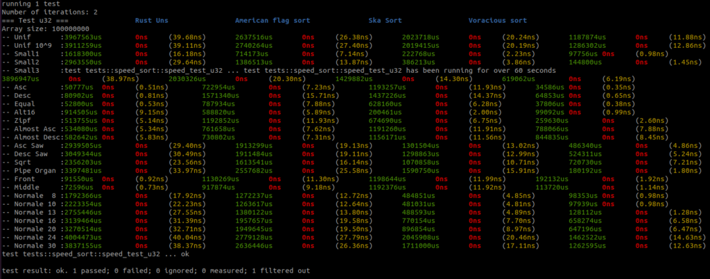
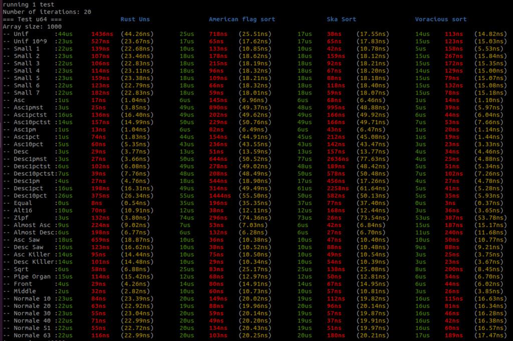
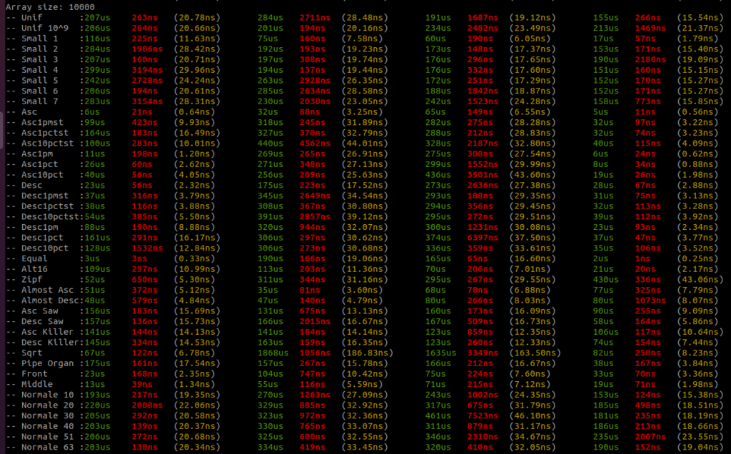
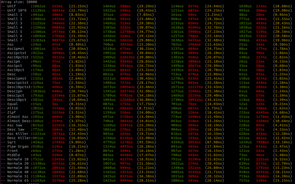
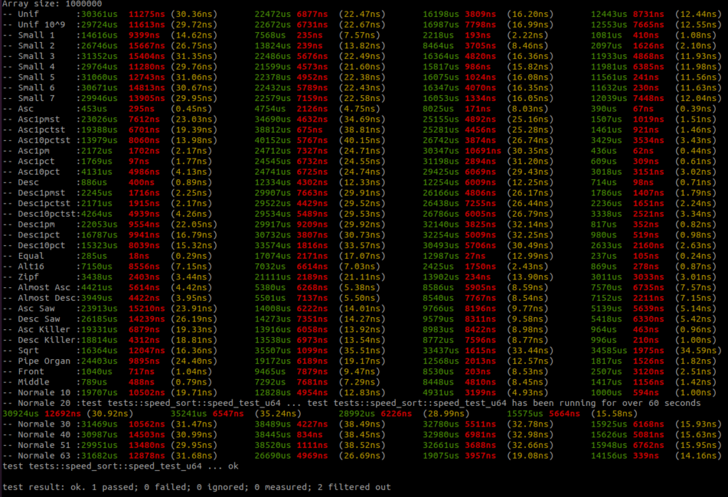
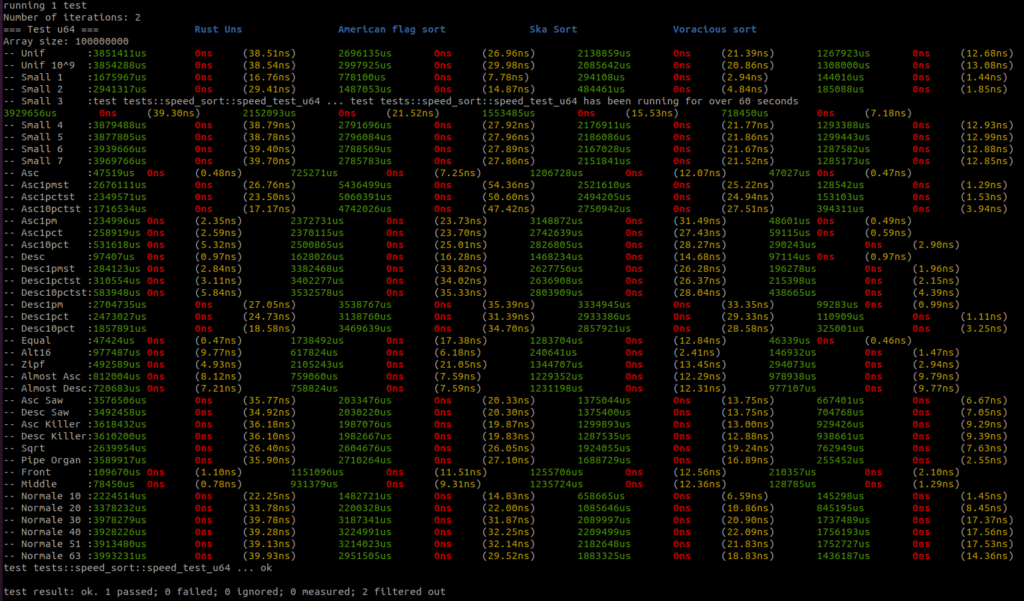
I added all the benchmark results here. There is a raw text file and all the screenshots.

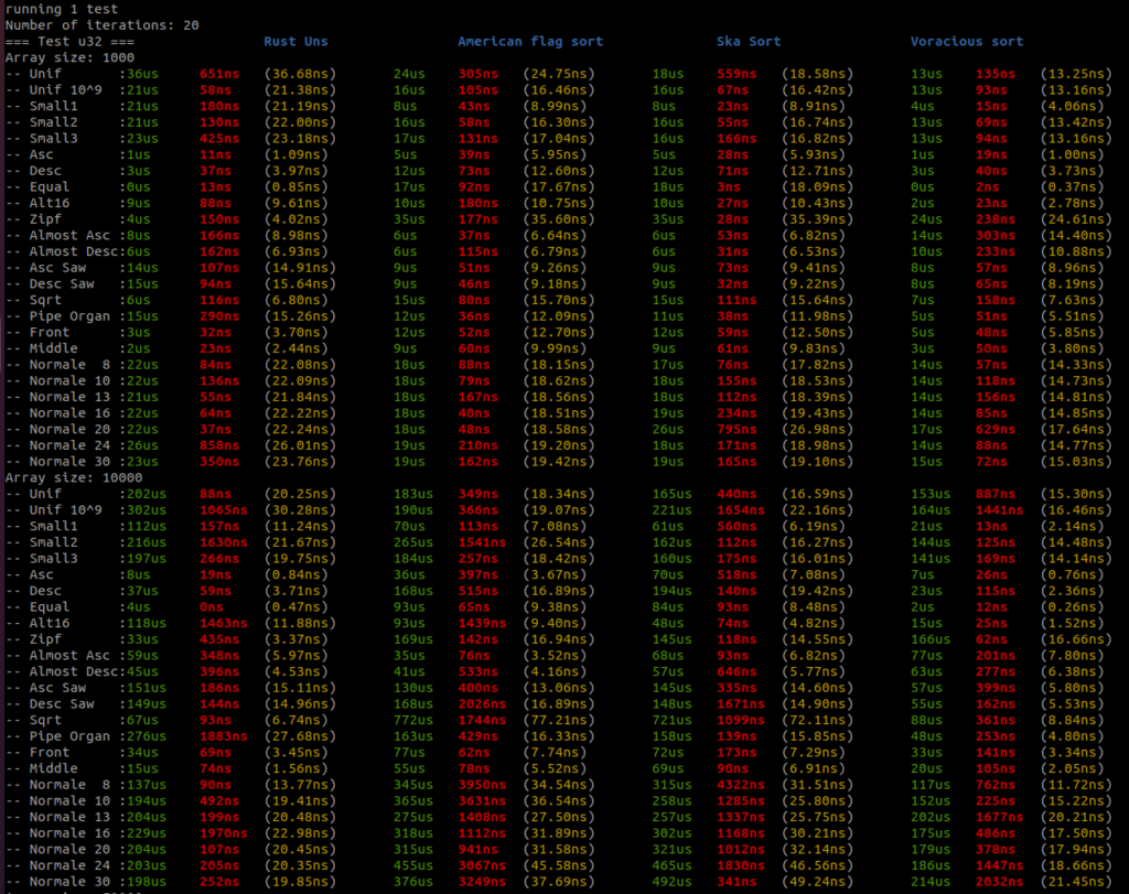
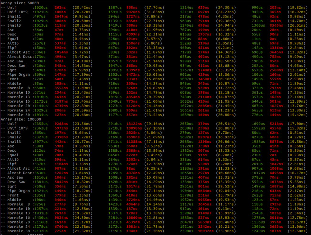
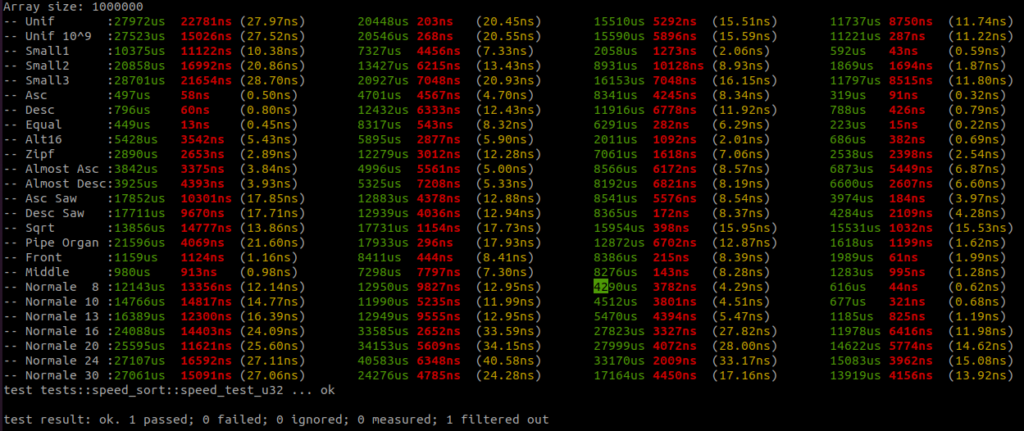
Benchmarks are done on an AMD Ryzen 9 3950x, 32GB RAM DDR4, MB X570 TUF Gaming.

For each sort there are three columns, the first column – green – is the running time in micro seconds, the second column – red – is the standard deviation if there is more than one round, and the third column – yellow – is the running time per item in nano seconds.

There are four sorts, the first sort is the Rust unstable_sort(): it is the Rust Pattern Defeating Quicksort. It is the current state of the art of the quicksort family and I guess the state of the art of the comparative sorts. Then there is the American flag sort, then the Rust Ska sort and then the Voracious sort.

I will let you analyse the results, but I take no risk in saying that the Voracious sort is the clear winner by far.

You can find all the data distribution generators here. So you can better understand what is tested. I wanted to have a sort that is faster than any other sorts on most of the data distributions so I implemented all the generators I could found. Too often, benchmark is done on too few data distributions and we don’t really grasp the sort efficiency for real cases in the real life.

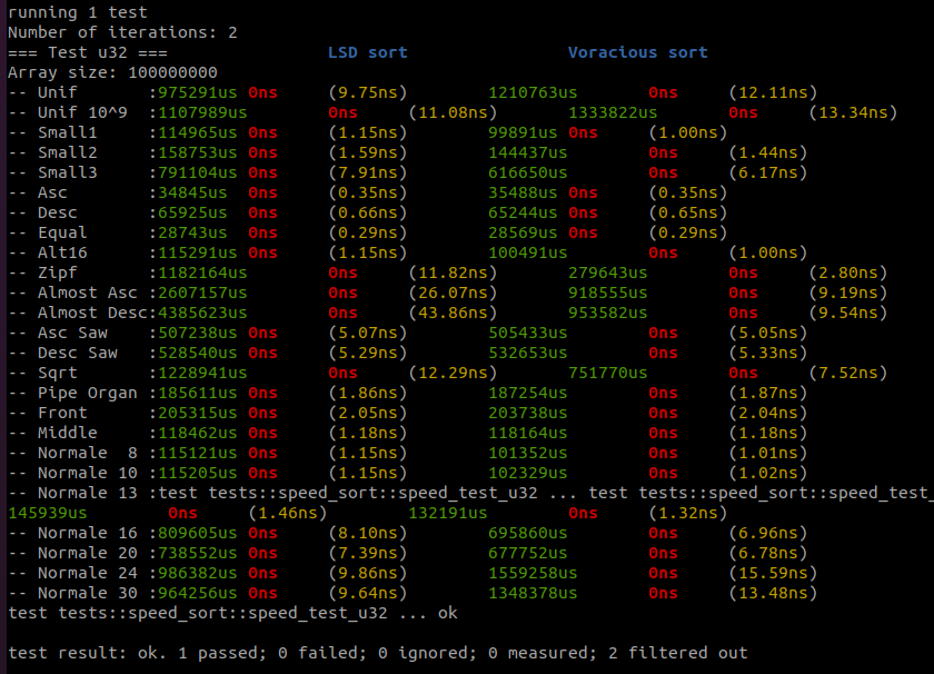
I haven’t added the benchmark on other type – i32, i64, f32, etc… -, because, it takes time to do all of this, and other researchers’ benchmarks rarely bother with other types. If you want more benchmark on the Rust Voracious Radix Sort Crate you can find them here. It is pretty exhaustive.

You have to understand that a sort can behave a particular way on a type and behave differently on another type. It is important to shape the sort for each type. It is not because the sort is efficient with unsigned integers that this very same sort will be efficient with signed integers or floats. I find it pretty sad that a lot of academic researchers only give benchmark results on unsigned integers.

Conclusion

We have seen, improvements after improvements, how I invented the Voracious sort and how it is implemented. Benchmark shows that Voracious sort is faster than the other sorts in the benchmarks on u32 and u64 on most of the data distributions.

Actually, Voracious sort is not the fastest sort I have, there are better sorts with respect to the element’s type. For example:

There are still lots to do. We have to explore the LSD radix sort approach and how it is possible to use diversion in a LSD sort – a.k.a. the DLSD sort -, and then how, with LSD and MSD sorts, I built the Rollercoaster sort. And finally, I will talk about the multithread sort Peeka sort, a challenger of the Regions sort from the MIT researchers.

See you soon.